Excel Quick Tip

Press "CTRL ~" to display all formulas.

Not only does this provide a quick view of the formula in the first cell, but it shows all formulas in the entire spreadsheet.  This can be used to quickly see information without having to scroll to the cell and view the formula in the formula bar.

Press "CTRL ~" again to hide the formulas and return to the standard view.

Excel 2007 Watch Window

If you're like many Excel fanatics, you probably deal with large spreadsheets and multiple cells containing formulas.

Excel 2007 has a great new feature that lets you "watch" cell contents as they change.  If numbers are added, subtracted, and changed, these specific cells are probably something you'd have to remember to review in previous versions of Excel.

To turn on the "Watch Window," follow these steps.

Highlight the cells you want to "Watch."

Click on the "Formula" tab and select the "Watch Window" button in the "Formula Auditing" group.

Click on the "Add Watch" button.

Since the cells were highlighted, simply click on the "OK" button and the cells will be added to the "Watch Window."



Now when you make changes to the spreadsheet, the "Watch Window" shows you the changes to the cells you added to the list.

If you accidentally close the "Watch Window," simply click on the "Formula" tab and then the "Watch Window" button to open it again.

Excel Cell Reference Tip

By default, Excel uses the "A1" format when referring to cells.  This means that the "A" is the Column and the "1" is the Row that is being referred to.  Most Excel users understand this; but some spreadsheet programs do not use this referencing.

Instead, other programs use the "R1C1" format when referencing cells.  Excel allows for this format as well.

To specify the format you want to use, follow these steps.

Excel 2007:

Click on the "Office" button and select the "Excel Options" button.

Select the "Formulas" tab on the left menu.

Check the "R1C1 reference style" checkbox in the "Working with Formulas" section and click the "OK" button to save the changes.



Excel 2003:
Click on the "Tools" menu and select the "Options" menu item.  Follow the above instructions from here.

Excel 2010:
Click on the "File" tab and select the "Excel Options" button.  Follow the above instructions from here.

Notice the Column Headers are now numbers instead of letters.



NOTE:  If you prefer the "A1" formatting and need to change Excel back to this preference, simply follow the above steps and uncheck the "R1C1" checkbox.

Change Gridline Colors in Excel 2007

This is a happy little feature that was added in Excel 2007.  Now you have the ability to change gridline colors in Excel 2007.

To do so, follow these steps:

Click on the "Office" button and click on the "Excel Options" button.

Select the "Advanced" tab from the left menu and scroll to the "Display Options for this Worksheet" area.  The gridline color option is located in the second section of "Display Options."

Click on the drop down to select a color.  Choose any color you want.

Click on the "OK" button to save the changes and exit the "Excel Options" window.

The gridline colors are now as you selected.

HINT: This may be helpful for situations where you have changed the background color to something light blue; thus, making the gridlines non-viewable.

Here's the caveat: only the selected worksheet is changed.  To change each sheet, you must select each sheet name from the drop down by the "Display Options" header and then change its corresponding color.

NOTE: Each new worksheet will display the gridline colors as the default light blue color.  You are not changing the default by selecting this option.

It's that simple to change gridline colors in Excel 2007.

Change Excel to International View

Intrenational users sometimes view things differently than here in the US.  But, did you know you can change Excel to International View?

Here's how:

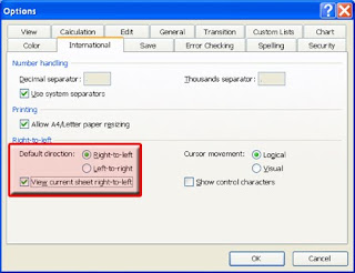
Click on the "Tools" menu and select "Options."

Click on the "International" tab and select the "Right to Left" checkbox.  If you want the current spreadsheet to change as well, click on the checkbox for "View current spreadsheet right to left" also.

All future spreadsheets will change to "Right to Left" view with Cell A1 on the right side of the screen as well as the row numbers.

To change it back, simply uncheck the above selections and click on the "Left to Right."

As always, make sure you click on the "OK" button to save the changes and close the "Options" window.

It's that simple!