Change Gridline Colors in Excel 2007

This is a happy little feature that was added in Excel 2007.  Now you have the ability to change gridline colors in Excel 2007.

To do so, follow these steps:

Click on the "Office" button and click on the "Excel Options" button.

Select the "Advanced" tab from the left menu and scroll to the "Display Options for this Worksheet" area.  The gridline color option is located in the second section of "Display Options."

Click on the drop down to select a color.  Choose any color you want.

Click on the "OK" button to save the changes and exit the "Excel Options" window.

The gridline colors are now as you selected.

HINT: This may be helpful for situations where you have changed the background color to something light blue; thus, making the gridlines non-viewable.

Here's the caveat: only the selected worksheet is changed.  To change each sheet, you must select each sheet name from the drop down by the "Display Options" header and then change its corresponding color.

NOTE: Each new worksheet will display the gridline colors as the default light blue color.  You are not changing the default by selecting this option.

It's that simple to change gridline colors in Excel 2007.

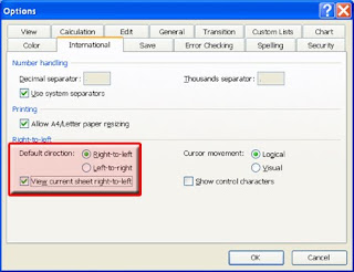
Change Excel to International View

Intrenational users sometimes view things differently than here in the US.  But, did you know you can change Excel to International View?

Here's how:

Click on the "Tools" menu and select "Options."

Click on the "International" tab and select the "Right to Left" checkbox.  If you want the current spreadsheet to change as well, click on the checkbox for "View current spreadsheet right to left" also.

All future spreadsheets will change to "Right to Left" view with Cell A1 on the right side of the screen as well as the row numbers.

To change it back, simply uncheck the above selections and click on the "Left to Right."

As always, make sure you click on the "OK" button to save the changes and close the "Options" window.

It's that simple!

How do I use AutoFilter in Excel?

Have you ever searched an entire Excel spreadsheet for data that matched certain criteria?

Use the AutoFilter in Excel and you will be able to find data much quicker.

To do so, simply follow these easy steps:

Excel 2007:
With your list open, click on the "Data" Tab on the Ribbon.  On the Data Tab, simply click the "Filter" button.

Notice your data Headers all have Drop Down Arrows next to them.

Now, simply click on the Drop Down Arrow of the Header (or Column) that contains the data in which you wish to search.

You may search for a specific item from the Drop Down list OR you may click on "Number Filters" from the Drop Down and another sub-menu will appear giving you options to search on items Greater than a particular number, etc.

Excel 2003:
Click on the Data Menu and choose "AutoFilter" and then follow the steps above.

It's that simple!