Go Ask Debbie: excel tutorial

Showing posts with label excel tutorial. Show all posts

How to Delete Blank Rows in Excel

This is the text version of a YouTube Live session of Go Ask Debbie: How to Delete Blank Rows in Excel.

I thought I'd just do a quick tip here to show people something that I've been often in Excel.

That is a lot of times when you start using data in Excel, you want to add formulas.

When you have a formula where there are blank rows, Excel stops at the first blank row, so your formula has to be manipulated a little bit - it's not so easy to calculate formulas.

So really when you're working with data in Excel, you want to get rid of all these blank rows.

They're not necessary. You may think that it looks nicer for formatting, but when you're trying to use Excel functions, really what Excel is for in calculating and manipulating data, you want to get rid of these rows.

So if the blank rows could be highlighted within your data, it's easy with a small list.

But if you have a large spreadsheet, Excel will recognize the blank rows without highlighting your data set.

But I'm going to go ahead and highlight this data set here.

Then you're going to go to your Home Tab,

and then over here on the right, you're going to click on the Find and Select button,

and then this time we're going to select Go to Special...

a pop-up window will appear

and you're simply going to select Blanks on the left-hand column and then hit OK.

You'll notice then that Excel highlights, in gray, all of the blank rows.

You'll see the first cell A4 is highlighted in white because that's the active cell.

But we really want to recognize these rows that are highlighted in gray.

These are truly all of our blank rows that we see on the screen here,

and to Delete those all in one swoop, we're just simply going to hit our CTRL key and then the Minus (-) sign.

Excel is going to open up another Dialog Box asking us to verify what we'd like to delete.

We want to delete the Entire Row for all these blank rows and then hit OK.

You'll see all the blank rows have disappeared, and now when I go to use Excel's function for Auto Sum, Excel knows exactly what I'd like to calculate.

There are no blank rows that are stopping the formula from calculating properly.

So again when we do this we're going to

Highlight our data set from our Home tab.
Click on Find and Select
and then Go to Special...
Click on Blanks
Hit the OK button
and then CTRL - (CTRL and Minus)
and select Entire Row
and OK

It really is that simple.

So now imagine if you've got a spreadsheet with tens of thousands of rows worth of data and you have 500 empty rows.

This makes it a lot faster than manually searching through blank rows and deleting them one at a time.

Thanks for taking this session of Go Ask Debbie with YouTube Live.

If you like what you see today, please Like the YouTube video.

Please feel free also to SUBSCRIBE to my channel to receive tips like this, and more, on a regular basis.

Please COMMENT if you have any other ideas for tutorials that you'd like to see on this channel.

Thanks for taking Go Ask Debbie and remember, be sure to SUBSCRIBE to my channel to continue seeing tips like this.

Thanks and everyone have a great day!

Watch the video here:

How to Calculate Percentages in Excel

Did you get your annual raise yet?

Many people have asked me over the years, "How do I calculate my annual raise when I know what percentage I'm getting?"

First, let's understand percentages. The term "percent" is literally broken down as "per," which means "out of" and "cent," which is one-hundred. So, a percent is the number out of one-hundred.

So, you're probably asking, "Debbie, how does that help me when I was told I was getting a 3% salary increase?"

Well, here's how you would calculate it.

Let's take Jim. Jim was told by his boss that he would be receiving a 3% salary increase on January 15th. If Jim's current salary is $40,000, let's see what his raise would be.

If you'd like to use Excel to do this, simply write the formula as such.

Column A would contain Jim's current salary of $40,000.

Column B would contain Jim's increase percentage of 3%.

Column C would calculate the 3% of $40,000, which would output $1,2000.

Column D would then add the $1,200 increase to Jim's current salary of $40,000, which would show his NEW Salary of $41,200.

Now, this is a bit of the long way around, but if it works for you, go ahead and use it.

For those of you who like quicker ways to calculate increases, here's what you would do. (Example shown in screenshot, Row 5)

Column A would contain Jim's current salary of $40,000.

Column B would contain the formula =A5*1.03 (this means you are saying I want 100% of the current salary, PLUS 3% added). This then gives you the $41,200 NEW Salary figure we came up with the 4 Column process above.

Hopefully, many of you will receive more than 3% with the new U.S. Tax Reform announced recently! But, this is just an example of how you can easily calculate percentages using Excel.

Please LIKE and COMMENT if you found this helpful.

Excel Macros Tutorial

For many years I've had students asking how to create Macros in Excel. So I created this Excel Macros Tutorial to show how you can create, setup, and use an Excel Macro in 3 Easy Steps.

If you have tasks in Microsoft Excel that you do repeatedly, you can record a macro to automate those tasks. A macro is an action or a set of actions that you can run as many times as you want.

When you create a macro, you are recording your mouse clicks and keystrokes. After you create a macro, you can edit it to make minor changes to the way it works.

Suppose that every month, you create a report for your manager. You want to sum the sales of the customers' revenue and apply bold formatting. You can create and then run a macro that quickly applies these formatting changes to the cells you select.

Here is the video showing you exactly that example:

As always, please Like, Comment, and Share my videos to keep them coming.

If you'd like tips like these and others, please SUBSCRIBE.

Thanks,
Debbie

Excel Tutorial: Named Ranges

When referencing data in larger Excel spreadsheets, it can often lead to incorrect results because of errors when selecting data. To avoid this, use Excel Named Ranges.

Here's a quick video to do just that.

It's really quite simple.

Excel Tutorial: How Can I Customize SmartArt?

Elizabeth asked, "Once I insert SmartArt in Excel, how can I change the color and look?"

What Elizabeth is asking is very smart. Inserting the same old SmartArt and not changing it, or customizing it in any way, looks very boring. I recommend customizing SmartArt and other objects to match your company colors and logo, your presentation style and format, so that it doesn't feel like it was an after thought.

To customize SmartArt, simply follow these steps.

You can also watch the video tutorial below.

Click the "Insert" Tab.
Click "SmartArt" from the Illustrations group.

In the "Choose a SmartArt Graphic" dialog box, select the category on the left. Then you select the item in the middle. The right shows a preview of the item. Select OK to insert the content.

Excel inserts the selected SmartArt graphic in the middle of the spreadsheet.

You can simply click on one of the boxes and type in your text, if desired. Notice that the font sizes adjust, depending on how much text you enter.

Don't stop there, now it's time to customize the SmartArt.

With the SmartArt selected (click on it, if you need), you will see the "SmartArt Tools" contextual tabs "Design" and "Format."

Click on these tabs to see the customization options. Features on these tabs will be different based on the type of SmartArt you inserted.

You can customize things like the colors, the styles, and fonts.

Look around and practice to find the best look for your Excel spreadsheet and/or presentation.

Now that you know how to customize SmartArt, you will look like the expert professional for visualizing in Excel.

Watch the video tutorial here.

Excel Tutorial: Auditing Formulas with Trace Precedents

If you have formulas that are based on the contents of another cell, you have precedent cells. If you have problems with a formula or result, you can trace the precedent cells to help track down the problem. The Trace Precedents command is useful to see the trail of data relationships. The Trace Precedents command allows you to show tracer arrows to show the relationship between the active cell and the precedents to that cell.

Tracer arrows are blue when pointing from a cell that provides data to another cell.
Red tracer arrows indicate an erroneous value.
Tracer arrows are black when pointing from a cell in another worksheet.
The other worksheet is represented by a worksheet icon.

If you prefer, watch the Video Tutorial below.

If tracer arrows do not show, you will need to turn on the objects in the Options window.

Use the following procedure.

Select the File Tab
Select Options.
Select the Advanced tab.
Under the Display options for this workbook, make sure the workbook you are using is displayed.
The For objects, show option should be All.

If a cell has a precedent that is in another worksheet, the other worksheet must be open.

For more tips like this, CLICK HERE to

download my FREE eBook:

65+ Ways to Use Office to be More Productive!

Excel Tutorial: Align Cells

In this Excel Tutorial: Align Cells, you'll learn the basic alignment techniques to make your data visually attractive. You'll also learn keyboard shortcuts for cell alignment.

If you prefer video, you may view the Excel Tutorial using the video below.

To align cells in Excel, it's quite simple.

Simply select the area you would like to align, typically this would be an entire column. If the entire column needs to be aligned a specific way, then click the Column Header to make the changes to the entire column.

Once the area is selected, click the alignment option you wish by using the "Alignment" area on the "Home" tab.

Options include:

Top, Middle, and Bottom Alignment for Vertical Alignment
Left, Center, and Right Alignment for Horizontal Alignment
Wrap Text to wrap the text within the cell
Merge and Center to merge data and center it across multiple cell

NOTE: Excel will give you a warning if you are merging data over existing data

And there are some indentation options as well

Here are a few keyboard shortcuts for these same functions to align cells:

CTRL + E = Center align
CTRL + J = Justify align
CTRL + L = Left align
CTRL + R = Right align

Watch this brief video tutorial, if you prefer.

I'm excited to announce my newest course - Excel Essentials: Tutorial for Beginners!

In this course, you will learn to use Excel in under 2 hours! We not only cover the basics, but teach useful Formulas, Functions, and Analysis.

I'm proud to offer my First 30 Fans with a Coupon to take the course for FREE!

Just CLICK HERE for the FREE Coupon.

Excel Essentials: Tutorial for Beginners Now Open

I'm proud to offer my First 30 Fans with a Coupon to take the course for FREE!

Just CLICK HERE for the FREE Coupon.

All I ask in return is that you write a review on the course.

Watch this quick preview of the course to learn more:

I hope you enjoy the course, and I know that you will learn valuable Excel skills.

Enjoy!
Debbie

How to Join Cells using Excel Concatenate

Excel Functions can seem overwhelming, but once they are broken down, they can be very easy, but can provide you with useful results.

Here's how to Join Cells using the Excel Function Concatenate.

You may read the steps here or view the video version below.

Do you need a Full Name field to import into a particular program? But, you only have First Name and Last Name fields in Excel? There are many times when you need to Merge or Join Cells in Excel - this tip shows you how easy it really is:

Insert a New Column.
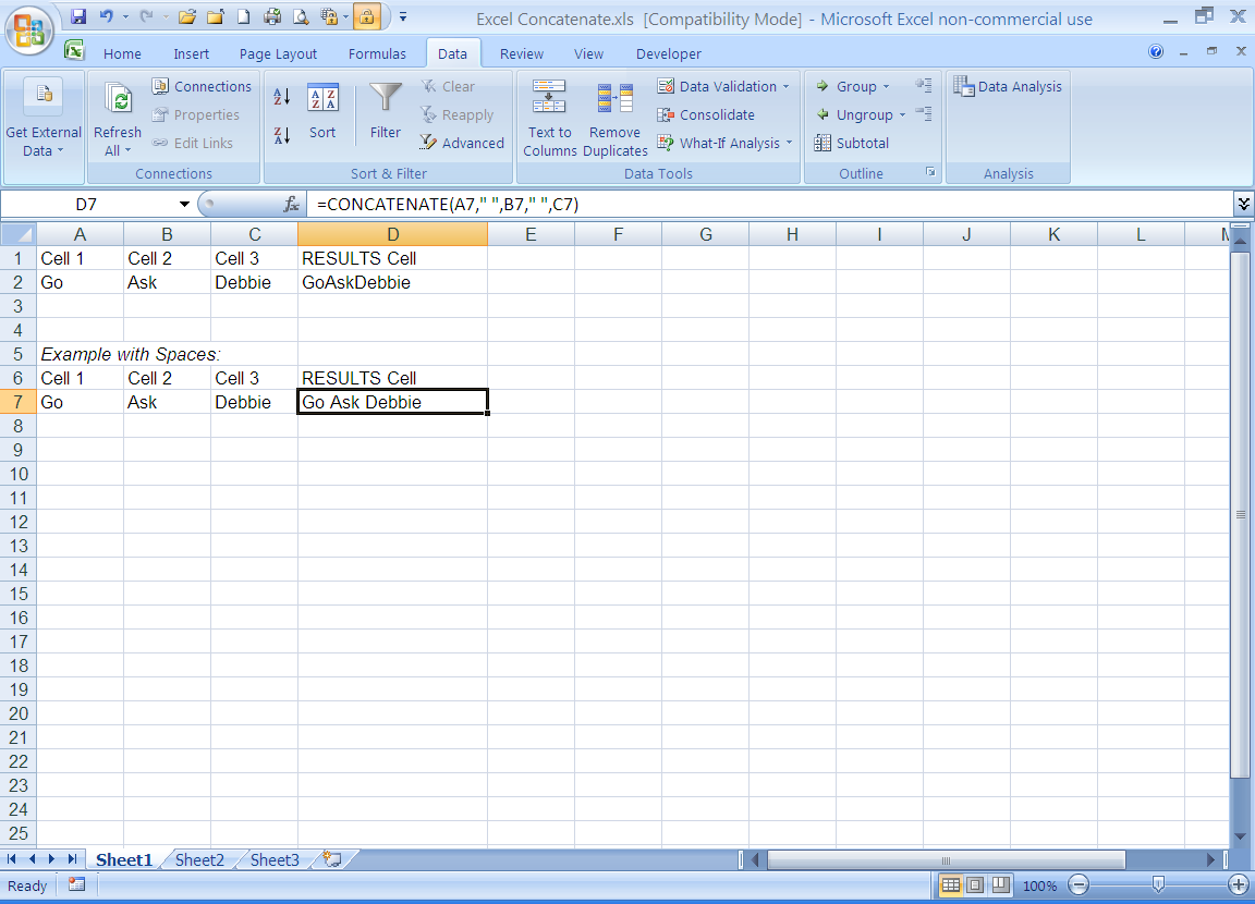
Type =CONCATENATE(Cell1,Cell2,etc)

Using the formula above, here is an example of the results:

Cell A1 Cell B1 Cell C1 RESULTS Cell D1
Go Ask Debbie GoAskDebbie

If these are the results you wish, simply Copy the formula down the column to include all rows you wish.

Let's say you need a Space or a Comma between each of the cells once they have been merged. To do this, type your formula as follows:

=CONCATENATE(Cell1," ",Cell2," ",etc.)

This would create the following result from the above scenario "Go Ask Debbie." Notice now there are spaces between the cell contents.

Go Ask Debbie