10 Tips You Didn’t Know You Could Do in Microsoft Outlook

Today, we’re diving into Microsoft Outlook and uncovering 10 awesome tips you probably didn’t know you could do. These tricks will help you streamline your workflow, stay organized, and boost your productivity. Let’s get started!

View on YouTube or Read below.

 

## 1. Schedule Emails to Send Later

 

Writing an email now but don’t want to interrupt someone’s day? Schedule it to send at the perfect time, ensuring your message lands when it’s most likely to be seen!

 

How to do it:

- Compose your email, then go to the “Options” tab.

- Click on “Delay Delivery.”

- Set your preferred date and time, and hit send!

 

## 2. Use Quick Steps for Routine Tasks

 

Automate repetitive actions to save time! Quick Steps allow you to execute multiple tasks with a single click, so you can focus on more important work.

 

How to set it up:

- Go to the “Home” tab and find the “Quick Steps” box.

- Click “Create New” and select your actions.

 

 

 

## 3. Clean Up Your Inbox with Clean Up Tool

 

Keep your inbox tidy! The Clean Up Tool helps you remove unnecessary emails from threads, making it easier to find important messages and reducing clutter.

 

Here’s how:

- Select the email conversation you want to clean.

- Click “Clean Up” in the Home tab.

- Choose “Clean Up Conversation.”

 

 

 

## 4. Create Rules for Automatic Email Management

 

Say goodbye to manual sorting! Create rules to automatically organize incoming emails, so you can spend less time managing your inbox and more time being productive.

 

To set it up:

- Go to “File” > “Manage Rules & Alerts.”

- Click “New Rule” and follow the prompts.

(Or, you may Right-click and select Rules, then Manage Rules & Alerts)

 

 

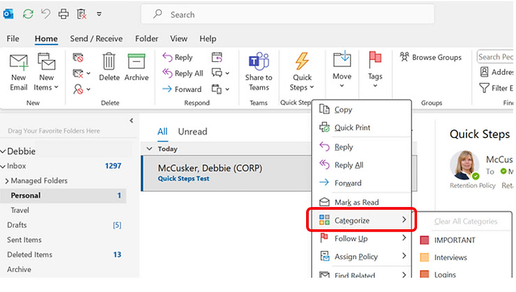
## 5. Use Categories for Better Organization

 

Easily prioritize your emails and tasks visually! Categorizing helps you quickly identify what needs your attention, keeping you focused and organized.

 

How to categorize:

- Right-click on an email, select “Categorize,” and choose a color or create a new category.

 

## 6. Keyboard Shortcuts for Faster Navigation

 

Navigate Outlook like a pro! Using keyboard shortcuts can drastically speed up your workflow, allowing you to accomplish tasks quicker without relying on your mouse.

 

Here are a few must-know ones:

- Ctrl + R: Reply to an email.

- Ctrl + N: Create a new email.

- Ctrl + Shift + M: Create a new message from anywhere in Outlook.

 

 

## 7.  Schedule Meetings Directly from Email

 

By turning an email thread into a meeting request with just a click, you save time and avoid the hassle of switching between different tools. This ensures clear communication, eliminates confusion about dates and times, and streamlines coordination with your team—all from the comfort of your inbox. You get to stay organized and efficient, focusing on what matters most without wasting time on back-and-forth scheduling.

 

When reading an email, click on the Meeting button (under the Home tab) to quickly turn an email thread into a meeting request.

 

 

## 8. Pin Important Emails

 

Keep essential messages front and center! Pinning important emails ensures that you always have quick access to critical information, making follow-ups easier.

 

How to do it:

- Right-click on the email and select “Pin.” It’ll stay at the top until you unpin it!

 

 

 

 

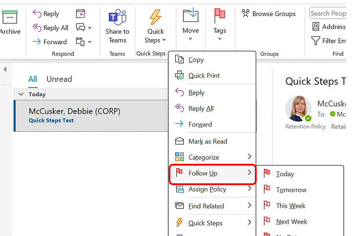
## 9. Set Reminders for Follow-Up

 

Never forget a follow-up! Setting reminders on emails ensures you stay on top of your commitments, helping you manage your time and responsibilities better.

 

Here’s how:

- Right-click on the email, select “Follow Up,” then choose a reminder date.

 

 

 

 

## 10. **Use Quick Parts to Insert Frequently Used Text*

With Quick Parts, you can quickly insert commonly used text, like responses, disclaimers, or greetings, into emai

ls without retyping or copying and pasting. This saves you time and effort, ensures consistency in your communication, and reduces the risk of mistakes. By streamlining repetitive tasks, you can focus on more important work and respond to emails faster, making your workflow more efficient and stress-free.

Save common text snippets with Quick Parts:

• Highlight the text in an email, go to the Insert tab, and select Quick Parts to save it for future use.

 

 

 

And there you have it—**10 fantastic tips for mastering Microsoft Outlook**! These features will not only save you time but also enhance your overall productivity. If you found these tips helpful, don’t forget to like, subscribe, and share your favorite Outlook hacks in the comments below!

 

See you next time, and happy emailing!

Thanks for your Support!

https://amzn.to/3Y0kRWP

Note: This post contains affiliate links, which means at no additional cost to you, we will receive a small commission if you make a purchase using the links. This helps support the channel and allows us to continue to make videos like this. Thank you for your support!

 6 Steps to Write with Clarity, so you are Heard

Write with Clarity and Conciseness

Writing with clarity and conciseness means to get right to the point. Write exactly what is meant without inserting double-speak and present content in the simplest terms possible.

Read below or watch the video here:

Six steps to write with clarity and conciseness:

1.       Organize key points before you write. You should already have performed this step when you ranked your key points or completed your planning worksheet. Either of these methods will provide you with a basic outline to write your communication and ensure that you stay focused on what you want to say, and keep your key points in the order you want to communicate them.

2.       Let your speech guide your writing. Try to write the way you would speak in normal, everyday conversation. However, do not be too informal. Do not use slang and abbreviations  - keep your writing on a professional level. Here are some tips to make your writing more reader friendly:

-         Use simple words. Avoid using a big word when a small one will do. Your readers will appreciate not having to go to a dictionary to look up the meaning of unfamiliar words.

-         Delete empty words. Avoid using a phrase when a word will do. Again, get to the point and reduce the time your readers need to spend to read your communication.

-         Trim rambling phrases. Long, rambling sentences with lots of punctuation marks can confuse your readers. You do not want your readers to get a headache trying to decode your message.

Get the Written Communication Skills Book here

3.       Avoid repetition and platitudes. Make your communications easy to read and understand. A repetition is a word, phrase or clause used more than once in a paragraph or short communication. A platitude is an unoriginal, overused declarative phrase. An example of a platitude is “There is no I in team.”

 

The example on the left below is filled with repetition and platitudes. The writer’s use of repetition and platitudes adds nothing to the message. In fact, the repetition and platitudes actually make it difficult to understand the results of the review and how they will help the customer.

The communication on the right has the repetitions and platitudes removed. Notice how much easier it is to read and comprehend the writer’s message. Also, notice how bullets are used to remove repetition and make the customer benefits clear and easy to see. 

4.       Use active voice to make your writing simple, direct, clear and easy to understand. Verbs have two voices: active voice and passive voice. In active voice, the person or thing acting is clear and specific. The doer or agent of the action comes before the action or verb. The active voice always makes clear “Who is doing, will do or had done what.” In the active voice examples below, Ed, we and the LMS system are the actors.

In passive voice, the writer does not specify who is acting or the writer specifies the actor later in the sentence. Avoid using passive voice because passive voice sentences are usually too wordy and weaken the clarity of your writing.

 

5.       Use action verbs to add clarity and power to your sentences. To put action in the verb, look for words that hide actions and change these words to action words (verbs). Many of these words end in “-tion,” and many are surrounded by “the,” “an” and “of.”

Compare these examples to see how putting the action in the verb makes a sentence more clear, strong and concise.

6.       Keep sentences to an average length between 15 to 28 words, depending on the type of document you are writing.

-         Emails, letters, memos and announcements: 15 and 22 words. An average shorter than 15 words per sentence means that your sentences are probably too choppy and do not flow well. The exception to this average is short email replies that may require less than 15 word responses.

-         Longer, more complicated documents (reports or proposals): 22 to 28. An average over 28 words means that your sentences are probably too wordy.

Compare the 53-word sentence to the revision below. The revision’s message is easier to read and understand because of shorter sentences, bullet points and unnecessary words are eliminated.

 

 

Perform the following steps to determine the average number of words in a sentence using the Word Count feature in Microsoft Word and Outlook.

Get the Written Communication Skills Book here

Excel Formulas, Functions, & PEMDAS

Welcome to this session Excel formulas and functions in this module we will learn how to perform basic calculations using formulas and functions.

The backbone of excel is its ability to perform calculations. Formulas are mathematical expressions that you build yourself you need to follow proper math principles in order to obtain the expected answer.

You may either watch the video here or follow the steps by reading the text in this blog located below.

To begin creating formulas and functions in Excel, you must understand basic math principles.

Basic arithmetic operators include the Plus Sign (+) which adds value, the Minus Sign (-) which subtracts value the Asterisk (*) which multiplies values the Forward Slash (/) which divides values the Percent Sign (%) which finds the percentage of a value and the carrot which finds the exponential value.

Basic comparison operators include the Equal Sign (=) which equates value, the Greater Than Sign (>) which indicates that one value is greater than the other, and the Less Than Sign (<) which indicates that one value is less than the other.

Let's review some of these.

Excel is like a calculator with simple formulas. Excel can perform calculations on numbers using operators we just talked about and functions such as Sum to add numbers.

The formula always starts with the Equal Sign(=) ,then type a number, then the plus sign, then another number and press Enter and the cell will display the results.

You can add many numbers this way, not just two. Instead of typing numbers in a formula, you can reference cells that contain the numbers to make adding easier and faster. It also gives you more more flexibility.

Let's create a formula that Adds the cells.

Type equals, click a cell, type the plus sign, then click another cell and press Enter.

If I change a number in one of the cells referenced, the results of the formula will automatically update.

When you double click a cell, you can see if the cell is a Formula. Double clicking or pressing F2 lets you see the contents of the cell. This places you in Edit mode for the cell. You can also see the contents in the formula bar here.

Subtracting is just like adding, but instead you use the minus sign, click a cell, then enter the minus sign, then another cell, and press Enter.

Multiplying and Dividing are similar.

To Multiply, use the Asterisk (*), press the equal sign, click a cell, then the asterisk, then another cell, then press enter.

To Divide use the Forward Slash (/), click a cell, press the forward slash, another cell, and then press enter.

AutoSum makes it easy to add adjacent cells in rows and columns.

You could type =A3 + A4+A5, etc, but that could be tedious with a large amount of data.

Instead, click the cell to the right of a row, or just below the column of where your data is housed, then on the Home tab click the AutoSum (Σ).

Confirm the formula is what you want to calculate and simply press Enter.

When I double-click the cell with the AutoSum you'll see it's a function. The syntax of the Sum function is =SUM(number1, number2, number3)

This formula is =SUM(A3:A6) which indicates a range of cells. It adds the cells from A3 through A6. If you try to do AutoSum here where there's missing data, it will only capture the adjacent cells with data, since row five is empty.

Excel doesn't recognize the entire column or group of adjacent cells to add cells and ranges of cells that aren't adjacent.

Type =SUM( and then hold the CTRL key and click the desired cells and ranges of cells, close parentheses and press Enter.

As a side note, the keyboard shortcut for AutoSum is ALT +.

Excel recognizes negative signs and it subtracts these numbers, even when using the Plus Sign for addition.

Excel uses the standard math order of operations you've probably heard PEMDAS, which stands for "Parentheses, Exponents, Multiplication, Division and last our Addition and Subtraction," all from left to right.

Excel understands and follows the order of operations, so when you write formulas, be sure to remember this rule as well.

Excel =VLOOKUP to quickly find data

Learn the power of Lookup Functions in Excel

 

Excel spreadsheets can become large and overwhelming at times. To manage large spreadsheets and find data easily, use the =VLOOKUP function as described in this tutorial.

Many people I've worked with over the years work have large spreadsheets containing hundreds and thousands of rows and columns worth of data. Often users manually search these hundreds or thousands of rows and columns to find specific data over and over again. This can be so time-consuming and has the potential for lots of errors.

 

But, when you need to find information in a large spreadsheet, there is an easier way. The =VLOOKUP function works quickly and easily.

=VLOOKUP works a lot like a phone book, where you start with the piece of data you know, like someone's name, in order to find out what you don't know, like their phone number.

Watch Video here or Continue to Read On...

To use the =VLOOKUP function, follow these steps.

For this example, use the Excel table in the image above. We've setup a table with the first column containing names of employees. The next few columns contain test scores pertaining to licensing information needed for the Human Resources department.

 

The Human Resources Director holds this data in an Excel spreadsheet and is asked to provide Dan's score on Test3.

 

The formula may be setup in a separate cell and edited to find specific information when needed. In our example, it would be very easy for the HR Director to simply find Dan's name in the "EMPLOYEE" column and look at the score for "Test 3." However, the =VLOOKUP function is really helpful when the spreadsheet contains hundreds or more rows and columns of data. So, pretend the data is so large that it's not obvious what Dan's score is on Test 3.

 

In Cell H2 we'll place the following formula:

 

=VLOOKUP("Dan",A2:F18,4,true)

 

Here is an explanation of each of the fields within the parentheses of the formula.

 

• "Dan" is the Lookup_Value. This is the data you are telling Excel to search.

• A2:F18 is the Table_Array. This is the range containing the data you want to search.

• 4 is the "Col_index_num" field. This is the number of the column that contains the data you need. In our example, "Test 3" scores are located in Column D, which is the 4th column in the spreadsheet.

• True is the "Range_lookup" field. This field defines how close a match should exist between the "Lookup_value" (Dan) and the value in the column on the lookup table. If Dan's name is listed as "Daniel," you may want to leave this field blank. When placing "false" in the "Range_lookup" field, Excel looks for an exact match to the "Lookup_value."

 

NOTE:  If Range_lookup is either "true" or is omitted, the values in the first column of Table_array must be placed in ascending sort order; otherwise, =VLOOKUP might not return the correct value.

 

So what just happened? I told Excel, “Here is a value in the left-hand column of my data - this is the name of the person I want to look up. Now look through this range of cells, and in the fourth column to the right (Test 3 data), find the value on the same row.”

The bottom line is that Excel spreadsheets containing large amounts of data do not need to be overwhelming and do not need to take a long time to find specific data. Use the =VLOOKUP function and your large Excel spreadsheets will become easy to manage.

 

Here's another example.

What if I wanted to keep the =VLOOKUP formula, but continue to use it to find results for different people based on what name I enter?

To do that, I'll simply need to replace the Lookup-Value reference. Instead of specifically entering "Dan" to find Dan, enter the field where you can enter a different name each time you'd like to search.

So, now the formula becomes =VLOOKUP(H1,A2:F18,4,True).

Now if we enter "Billy" into cell H1, the result provides us Billy's score of 88.

If we then change H1 by entering "Dan," we now see Dan's Test 3 score of 78 again.

Now, practice on your own. What if you wanted to change the Test # you want to search for?

The examples here are so powerful, but as you can now imagine, =VLOOKUP can be so powerful and helpful. I urge you to try this for a basic search of data you have in a spreadsheet and as you get more and more comfortable with =VLOOKUP, try to push it like we started in the second example here.

Good Luck and Happy Excelling!

Excel: Create a Pivot Chart from Pivot Table

In this tutorial, I show you how to easily create a Pivot Chart from an existing Pivot Table.

Continue below to read or watch the video here.

Creating a Pivot Chart from a Pivot Table

Click anywhere in the PivotTable for which you want to add a chart.

1.       Select the Options tab from the Ribbon.

2.       Select PivotChart.

Excel displays the Insert Chart dialog box.

3.       Select the desired type of chart and select OK.

Creating a Pivot Chart from Data

Use the following procedure to insert a PivotChart.

1.       Place your cursor somewhere in the data you want to analyze.

2.       Select the Insert tab from the Ribbon.

3.       Select the arrow under PivotTable. Select PivotChart.

Excel displays the Create PivotTable with PivotChart dialog box.

4.       Excel automatically provides a range of cells based on your selection. You can change the table or range if desired.

5.       Select a location for the PivotChart. You can have Excel create a new worksheet or select one of the existing sheets.

6.       Select OK.

Excel displays the PivotChart and the Field List for you to begin choosing your fields and grouping data.

7.       Add fields to view the chart.

Excel Macros for Productivity

#Excel, #ExcelProductivity, #ExcelTraining, #ExcelTutorial, #ExcelMacros

Macros in Excel can tremendously help with your productivity!

Macros, in essence, record steps you would conduct on a regular basis in Excel. And then, Excel performs the entire set of steps when you tell it to.

When I first learned Macros was many years ago when I had to run multiple reports each and every month. It basically turned about 2 weeks worth of work into about 2 days!

And many of my students have had similar results by just learning how to setup and use Excel Macros.

For a full tutorial on how to use Macros in 3 Easy Steps, CLICK HERE.

Lately, I've had quite a few students saying their macros has disappeared. I've had this happen to me over the years as well and found this amazingly helpful tip.

To make sure you always have access to your Macros, copy them to a Personal Macro Workbook.

If you find yourself recreating the same macros, you can copy those macros to a special workbook called Personal.xlsb that is saved on your computer. Any macros that you store in your personal workbook become available to you whenever you start Excel on that same computer.

This is different than Excel's default behavior, where a macro only works in the workbook that contains it.

To create the personal workbook, you first need to create a macro and store it in the Personal Macro Workbook. Before you get started, make sure that the Developer tab is available in the ribbon in Excel.

Create and update the Personal Macro workbook by following these steps:

• On the Developer tab, in the Code group, click Record Macro.

• In the Record Macro dialog box, type a meaningful name for the macro in the Macro name box. Make sure you don’t use any spaces in the name.

• In the Store macro in box, select Personal Macro Workbook.
  

• Click OK.

• Perform the actions that you want to record. (Meaning, perform the steps that you would normally perform that are repetitive. For example, every month, I used to create a report from a data set that would create Pivot Tables, Sum and Average data, and format in a specific manner. All of those things are the actions that I want to record so that I do not have to repeat them each and every month).

• On the Developer tab, in the Code group, click Stop Recording.
  

• Close the workbook.
  A message appears that prompts you to save the changes that you made to the Personal Macro Workbook.

• Click Save to save the workbook.

Any time you create a new macro and save it in your personal workbook or update any macros that it contains, you are prompted to save the personal workbook just as it did the first time you saved it.

Next time you need to run a Macro, it is now saved in the Personal Macro Workbook!